diatomic-py

Python package to calculate the hyperfine energy levels of singlet sigma diatomic molecules (e.g. RbCs, KCs and KRb) under various applied fields. The hyperfine structure can be calculated in static electric and magnetic fields and, when provided the polarisability, oscillating electric fields.

More detailed information can be found in the documentation at https://diatomic-py.readthedocs.io .

Diatomic-py is licensed under a BSD 3 clause license, a copy can be found here.

If you use our work for academic purposes you can cite us using:

J.A.Blackmore et al. Diatomic-py: A python module for calculating the rotational and hyperfine structure of \(^1\Sigma\) molecules, [Arxiv e-prints 2205.05686](https://arxiv.org/abs/2205.05686) (2022).

This work has continued to evolve since the release of the paper, and so the API is different.

PyPi Installation

python -m pip install diatomic-py

Manual Installation

Clone the repository:

git clone https://github.com/durham-qlm/diatomic-py.git
cd diatomic-py

It is recommended to then install the python package into virtual environment:

# You may need to substitute `python` for `python3` if you're on macOS
python -m venv ./venv
source ./venv/bin/activate
# After activating the virtual env you should only need `python`
python --version
which python

The below installation commands assume you are active in such an environment. You can then install the package, there are various options indicated inside the square brackets for the command types:

# Installs essentials + matplotlib
python -m pip install ".[plotting]"

# OR if you also want to run test suite:
python -m pip install ".[test,plotting]"
pytest

# OR if you want to develop code for the package
python -m pip install -e ".[dev,plotting]"
pre-commit install

Example

import numpy as np
import matplotlib.pyplot as plt
import scipy.constants

from diatomic.systems import SingletSigmaMolecule
import diatomic.operators as operators
import diatomic.calculate as solver

GAUSS = 1e-4  # T
MHz = scipy.constants.h * 1e6

# Generate Molecule
mol = SingletSigmaMolecule.from_preset("Rb87Cs133")
mol.Nmax = 2

# Generate Hamiltonians
H0 = operators.hyperfine_ham(mol)
Hz = operators.zeeman_ham(mol)

# Parameter Space
B = np.linspace(0.001, 300, 50) * GAUSS

# Overall Hamiltonian
Htot = H0 + Hz * B[:, None, None]

# Solve (diagonalise) Hamiltonians
eigenenergies, eigenstates = solver.solve_system(Htot)

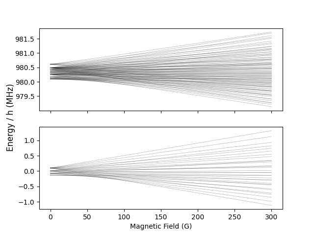
# Plot results
fig, (ax_up, ax_down) = plt.subplots(2, 1, sharex=True)

ax_down.plot(B / GAUSS, eigenenergies[:, 0:32] / MHz, c="k", lw=0.5, alpha=0.3)
ax_up.plot(B / GAUSS, eigenenergies[:, 32:128] / MHz, c="k", lw=0.5, alpha=0.3)

ax_down.set_xlabel("Magnetic Field (G)")
fig.supylabel("Energy / h (MHz)")

plt.show()

For more examples of usage, see the ./examples folder.